Prediction (out of sample)
[1]:
%matplotlib inline
[2]:
import numpy as np
import matplotlib.pyplot as plt

import statsmodels.api as sm

plt.rc("figure", figsize=(16, 8))
plt.rc("font", size=14)
Artificial data
[3]:
nsample = 50
sig = 0.25
x1 = np.linspace(0, 20, nsample)
X = np.column_stack((x1, np.sin(x1), (x1 - 5) ** 2))
X = sm.add_constant(X)
beta = [5.0, 0.5, 0.5, -0.02]
y_true = np.dot(X, beta)
y = y_true + sig * np.random.normal(size=nsample)
Estimation
[4]:
olsmod = sm.OLS(y, X)
olsres = olsmod.fit()
print(olsres.summary())
                            OLS Regression Results
==============================================================================
Dep. Variable:                      y   R-squared:                       0.982
Model:                            OLS   Adj. R-squared:                  0.981
Method:                 Least Squares   F-statistic:                     824.9
Date:                Mon, 10 Jun 2024   Prob (F-statistic):           5.56e-40
Time:                        11:17:13   Log-Likelihood:               -0.64591
No. Observations:                  50   AIC:                             9.292
Df Residuals:                      46   BIC:                             16.94
Df Model:                           3
Covariance Type:            nonrobust
==============================================================================
                 coef    std err          t      P>|t|      [0.025      0.975]
------------------------------------------------------------------------------
const          5.0685      0.087     58.190      0.000       4.893       5.244
x1             0.4805      0.013     35.766      0.000       0.453       0.507
x2             0.5155      0.053      9.761      0.000       0.409       0.622
x3            -0.0187      0.001    -15.820      0.000      -0.021      -0.016
==============================================================================
Omnibus:                        0.273   Durbin-Watson:                   1.301
Prob(Omnibus):                  0.873   Jarque-Bera (JB):                0.367
Skew:                          -0.162   Prob(JB):                        0.832
Kurtosis:                       2.732   Cond. No.                         221.
==============================================================================

Notes:
[1] Standard Errors assume that the covariance matrix of the errors is correctly specified.
In-sample prediction
[5]:
ypred = olsres.predict(X)
print(ypred)
[ 4.60204018  5.07579939  5.5097256   5.87572593  6.1558461   6.34522021
  6.45287024  6.50022372  6.5175933   6.53919642  6.5975335   6.71804822
  6.91494719  7.18886582  7.52676398  7.90406841  8.28871003  8.64639285
  8.94622866  9.16581187  9.29490074  9.33710001  9.30926867  9.2387501
  9.15887958  9.10350746  9.10143759  9.17169495  9.32039992  9.53976266
  9.80936304 10.09950554 10.37609816 10.60625368 10.76369287 10.83306213
 10.81245606 10.71373046 10.56055452 10.38452198 10.21996039 10.09829123
 10.04286736 10.06513632 10.16275943 10.31999611 10.51028996 10.70063191
 10.85698356 10.94986951]
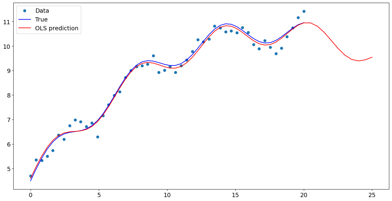
Create a new sample of explanatory variables Xnew, predict and plot
[6]:
x1n = np.linspace(20.5, 25, 10)
Xnew = np.column_stack((x1n, np.sin(x1n), (x1n - 5) ** 2))
Xnew = sm.add_constant(Xnew)
ynewpred = olsres.predict(Xnew)  # predict out of sample
print(ynewpred)
[10.94878329 10.81256159 10.56141937 10.24142388  9.91321585  9.63716252
  9.45857761  9.39662696  9.43963605  9.54794836]
Plot comparison
[7]:
import matplotlib.pyplot as plt

fig, ax = plt.subplots()
ax.plot(x1, y, "o", label="Data")
ax.plot(x1, y_true, "b-", label="True")
ax.plot(np.hstack((x1, x1n)), np.hstack((ypred, ynewpred)), "r", label="OLS prediction")
ax.legend(loc="best")
[7]:
<matplotlib.legend.Legend at 0x7f5a8ae4fc10>
Predicting with Formulas
Using formulas can make both estimation and prediction a lot easier
[8]:
from statsmodels.formula.api import ols

data = {"x1": x1, "y": y}

res = ols("y ~ x1 + np.sin(x1) + I((x1-5)**2)", data=data).fit()
We use the I to indicate use of the Identity transform. Ie., we do not want any expansion magic from using **2
[9]:
res.params
[9]:
Intercept           5.068521
x1                  0.480454
np.sin(x1)          0.515474
I((x1 - 5) ** 2)   -0.018659
dtype: float64
Now we only have to pass the single variable and we get the transformed right-hand side variables automatically
[10]:
res.predict(exog=dict(x1=x1n))
[10]:
0    10.948783
1    10.812562
2    10.561419
3    10.241424
4     9.913216
5     9.637163
6     9.458578
7     9.396627
8     9.439636
9     9.547948
dtype: float64
Last update:
Jun 10, 2024