Robust Linear Models
[1]:
%matplotlib inline
[2]:
import matplotlib.pyplot as plt
import numpy as np
import statsmodels.api as sm
Estimation
Load data:
[3]:
data = sm.datasets.stackloss.load()
data.exog = sm.add_constant(data.exog)
Huber’s T norm with the (default) median absolute deviation scaling
[4]:
huber_t = sm.RLM(data.endog, data.exog, M=sm.robust.norms.HuberT())
hub_results = huber_t.fit()
print(hub_results.params)
print(hub_results.bse)
print(
    hub_results.summary(
        yname="y", xname=["var_%d" % i for i in range(len(hub_results.params))]
    )
)
const       -41.026498
AIRFLOW       0.829384
WATERTEMP     0.926066
ACIDCONC     -0.127847
dtype: float64
const        9.791899
AIRFLOW      0.111005
WATERTEMP    0.302930
ACIDCONC     0.128650
dtype: float64
                    Robust linear Model Regression Results
==============================================================================
Dep. Variable:                      y   No. Observations:                   21
Model:                            RLM   Df Residuals:                       17
Method:                          IRLS   Df Model:                            3
Norm:                          HuberT
Scale Est.:                       mad
Cov Type:                          H1
Date:                Mon, 10 Jun 2024
Time:                        11:13:41
No. Iterations:                    19
==============================================================================
                 coef    std err          z      P>|z|      [0.025      0.975]
------------------------------------------------------------------------------
var_0        -41.0265      9.792     -4.190      0.000     -60.218     -21.835
var_1          0.8294      0.111      7.472      0.000       0.612       1.047
var_2          0.9261      0.303      3.057      0.002       0.332       1.520
var_3         -0.1278      0.129     -0.994      0.320      -0.380       0.124
==============================================================================

If the model instance has been used for another fit with different fit parameters, then the fit options might not be the correct ones anymore .
Huber’s T norm with ‘H2’ covariance matrix
[5]:
hub_results2 = huber_t.fit(cov="H2")
print(hub_results2.params)
print(hub_results2.bse)
const       -41.026498
AIRFLOW       0.829384
WATERTEMP     0.926066
ACIDCONC     -0.127847
dtype: float64
const        9.089504
AIRFLOW      0.119460
WATERTEMP    0.322355
ACIDCONC     0.117963
dtype: float64
Andrew’s Wave norm with Huber’s Proposal 2 scaling and ‘H3’ covariance matrix
[6]:
andrew_mod = sm.RLM(data.endog, data.exog, M=sm.robust.norms.AndrewWave())
andrew_results = andrew_mod.fit(scale_est=sm.robust.scale.HuberScale(), cov="H3")
print("Parameters: ", andrew_results.params)
Parameters:  const       -40.881796
AIRFLOW       0.792761
WATERTEMP     1.048576
ACIDCONC     -0.133609
dtype: float64
See help(sm.RLM.fit) for more options and module sm.robust.scale for scale options
Comparing OLS and RLM
Artificial data with outliers:
[7]:
nsample = 50
x1 = np.linspace(0, 20, nsample)
X = np.column_stack((x1, (x1 - 5) ** 2))
X = sm.add_constant(X)
sig = 0.3  # smaller error variance makes OLS<->RLM contrast bigger
beta = [5, 0.5, -0.0]
y_true2 = np.dot(X, beta)
y2 = y_true2 + sig * 1.0 * np.random.normal(size=nsample)
y2[[39, 41, 43, 45, 48]] -= 5  # add some outliers (10% of nsample)
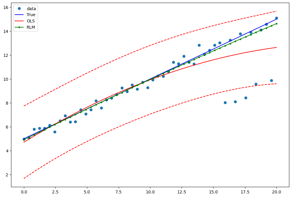
Example 1: quadratic function with linear truth
Note that the quadratic term in OLS regression will capture outlier effects.
[8]:
res = sm.OLS(y2, X).fit()
print(res.params)
print(res.bse)
print(res.predict())
[ 5.01677648  0.52266348 -0.01259729]
[0.46634628 0.07199757 0.00637067]
[ 4.70184419  4.96449506  5.22294859  5.47720477  5.7272636   5.97312509
  6.21478922  6.45225601  6.68552545  6.91459754  7.13947228  7.36014967
  7.57662972  7.78891241  7.99699776  8.20088576  8.40057641  8.59606972
  8.78736567  8.97446428  9.15736554  9.33606945  9.51057601  9.68088522
  9.84699709 10.0089116  10.16662877 10.32014859 10.46947106 10.61459619
 10.75552396 10.89225439 11.02478747 11.1531232  11.27726158 11.39720261
 11.5129463  11.62449263 11.73184162 11.83499326 11.93394755 12.0287045
 12.11926409 12.20562634 12.28779123 12.36575878 12.43952899 12.50910184
 12.57447734 12.6356555 ]
Estimate RLM:
[9]:
resrlm = sm.RLM(y2, X).fit()
print(resrlm.params)
print(resrlm.bse)
[ 4.95750107e+00  5.05398579e-01 -1.92991202e-03]
[0.15151367 0.02339167 0.0020698 ]
Draw a plot to compare OLS estimates to the robust estimates:
[10]:
fig = plt.figure(figsize=(12, 8))
ax = fig.add_subplot(111)
ax.plot(x1, y2, "o", label="data")
ax.plot(x1, y_true2, "b-", label="True")
pred_ols = res.get_prediction()
iv_l = pred_ols.summary_frame()["obs_ci_lower"]
iv_u = pred_ols.summary_frame()["obs_ci_upper"]

ax.plot(x1, res.fittedvalues, "r-", label="OLS")
ax.plot(x1, iv_u, "r--")
ax.plot(x1, iv_l, "r--")
ax.plot(x1, resrlm.fittedvalues, "g.-", label="RLM")
ax.legend(loc="best")
[10]:
<matplotlib.legend.Legend at 0x7f270cf73cd0>
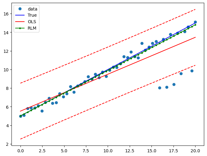
Example 2: linear function with linear truth
Fit a new OLS model using only the linear term and the constant:
[11]:
X2 = X[:, [0, 1]]
res2 = sm.OLS(y2, X2).fit()
print(res2.params)
print(res2.bse)
[5.52452446 0.39669057]
[0.40091385 0.03454436]
Estimate RLM:
[12]:
resrlm2 = sm.RLM(y2, X2).fit()
print(resrlm2.params)
print(resrlm2.bse)
[5.02153867 0.48893671]
[0.12418732 0.01070048]
Draw a plot to compare OLS estimates to the robust estimates:
[13]:
pred_ols = res2.get_prediction()
iv_l = pred_ols.summary_frame()["obs_ci_lower"]
iv_u = pred_ols.summary_frame()["obs_ci_upper"]

fig, ax = plt.subplots(figsize=(8, 6))
ax.plot(x1, y2, "o", label="data")
ax.plot(x1, y_true2, "b-", label="True")
ax.plot(x1, res2.fittedvalues, "r-", label="OLS")
ax.plot(x1, iv_u, "r--")
ax.plot(x1, iv_l, "r--")
ax.plot(x1, resrlm2.fittedvalues, "g.-", label="RLM")
legend = ax.legend(loc="best")
Last update:
Jun 10, 2024