VARMAX models
This is a brief introduction notebook to VARMAX models in statsmodels. The VARMAX model is generically specified as:
where \(y_t\) is a \(\text{k_endog} \times 1\) vector.
[1]:
%matplotlib inline
[2]:
import numpy as np
import pandas as pd
import statsmodels.api as sm
import matplotlib.pyplot as plt
[3]:
import requests
import shutil

def download_file(url):
    local_filename = url.split('/')[-1]
    with requests.get(url, stream=True) as r:
        with open(local_filename, 'wb') as f:
            shutil.copyfileobj(r.raw, f)

    return local_filename

filename = download_file("https://www.stata-press.com/data/r12/lutkepohl2.dta")

dta = pd.read_stata(filename)
dta.index = dta.qtr
dta.index.freq = dta.index.inferred_freq
endog = dta.loc['1960-04-01':'1978-10-01', ['dln_inv', 'dln_inc', 'dln_consump']]
Model specification
The VARMAX class in statsmodels allows estimation of VAR, VMA, and VARMA models (through the order argument), optionally with a constant term (via the trend argument). Exogenous regressors may also be included (as usual in statsmodels, by the exog argument), and in this way a time trend may be added. Finally, the class allows measurement error (via the measurement_error argument) and allows specifying either a diagonal or unstructured innovation covariance matrix (via the
error_cov_type argument).
Example 1: VAR
Below is a simple VARX(2) model in two endogenous variables and an exogenous series, but no constant term. Notice that we needed to allow for more iterations than the default (which is maxiter=50) in order for the likelihood estimation to converge. This is not unusual in VAR models which have to estimate a large number of parameters, often on a relatively small number of time series: this model, for example, estimates 27 parameters off of 75 observations of 3 variables.
[4]:
exog = endog['dln_consump']
mod = sm.tsa.VARMAX(endog[['dln_inv', 'dln_inc']], order=(2,0), trend='n', exog=exog)
res = mod.fit(maxiter=1000, disp=False)
print(res.summary())
                             Statespace Model Results
==================================================================================
Dep. Variable:     ['dln_inv', 'dln_inc']   No. Observations:                   75
Model:                            VARX(2)   Log Likelihood                 361.037
Date:                    Mon, 10 Jun 2024   AIC                           -696.074
Time:                            11:12:31   BIC                           -665.946
Sample:                        04-01-1960   HQIC                          -684.044
                             - 10-01-1978
Covariance Type:                      opg
===================================================================================
Ljung-Box (L1) (Q):            0.04, 10.22   Jarque-Bera (JB):          11.10, 2.44
Prob(Q):                        0.84, 0.00   Prob(JB):                   0.00, 0.30
Heteroskedasticity (H):         0.45, 0.40   Skew:                      0.16, -0.38
Prob(H) (two-sided):            0.05, 0.03   Kurtosis:                   4.86, 3.44
                            Results for equation dln_inv
====================================================================================
                       coef    std err          z      P>|z|      [0.025      0.975]
------------------------------------------------------------------------------------
L1.dln_inv          -0.2424      0.093     -2.618      0.009      -0.424      -0.061
L1.dln_inc           0.2827      0.448      0.631      0.528      -0.595       1.161
L2.dln_inv          -0.1621      0.155     -1.045      0.296      -0.466       0.142
L2.dln_inc           0.0816      0.421      0.194      0.846      -0.744       0.907
beta.dln_consump     0.9634      0.637      1.513      0.130      -0.285       2.212
                            Results for equation dln_inc
====================================================================================
                       coef    std err          z      P>|z|      [0.025      0.975]
------------------------------------------------------------------------------------
L1.dln_inv           0.0622      0.036      1.732      0.083      -0.008       0.133
L1.dln_inc           0.0824      0.107      0.768      0.443      -0.128       0.293
L2.dln_inv           0.0093      0.033      0.282      0.778      -0.055       0.074
L2.dln_inc           0.0328      0.134      0.244      0.807      -0.230       0.296
beta.dln_consump     0.7754      0.112      6.905      0.000       0.555       0.995
                                  Error covariance matrix
============================================================================================
                               coef    std err          z      P>|z|      [0.025      0.975]
--------------------------------------------------------------------------------------------
sqrt.var.dln_inv             0.0433      0.004     12.327      0.000       0.036       0.050
sqrt.cov.dln_inv.dln_inc  3.564e-05      0.002      0.018      0.986      -0.004       0.004
sqrt.var.dln_inc             0.0109      0.001     11.202      0.000       0.009       0.013
============================================================================================

Warnings:
[1] Covariance matrix calculated using the outer product of gradients (complex-step).
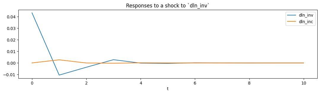
From the estimated VAR model, we can plot the impulse response functions of the endogenous variables.
[5]:
ax = res.impulse_responses(10, orthogonalized=True, impulse=[1, 0]).plot(figsize=(13,3))
ax.set(xlabel='t', title='Responses to a shock to `dln_inv`');
Example 2: VMA
A vector moving average model can also be formulated. Below we show a VMA(2) on the same data, but where the innovations to the process are uncorrelated. In this example we leave out the exogenous regressor but now include the constant term.
[6]:
mod = sm.tsa.VARMAX(endog[['dln_inv', 'dln_inc']], order=(0,2), error_cov_type='diagonal')
res = mod.fit(maxiter=1000, disp=False)
print(res.summary())
                             Statespace Model Results
==================================================================================
Dep. Variable:     ['dln_inv', 'dln_inc']   No. Observations:                   75
Model:                             VMA(2)   Log Likelihood                 353.880
                              + intercept   AIC                           -683.760
Date:                    Mon, 10 Jun 2024   BIC                           -655.951
Time:                            11:12:54   HQIC                          -672.656
Sample:                        04-01-1960
                             - 10-01-1978
Covariance Type:                      opg
===================================================================================
Ljung-Box (L1) (Q):             0.00, 0.03   Jarque-Bera (JB):         13.31, 14.48
Prob(Q):                        0.99, 0.86   Prob(JB):                   0.00, 0.00
Heteroskedasticity (H):         0.44, 0.80   Skew:                      0.06, -0.50
Prob(H) (two-sided):            0.04, 0.59   Kurtosis:                   5.06, 4.91
                           Results for equation dln_inv
=================================================================================
                    coef    std err          z      P>|z|      [0.025      0.975]
---------------------------------------------------------------------------------
intercept         0.0182      0.005      3.795      0.000       0.009       0.028
L1.e(dln_inv)    -0.2502      0.106     -2.359      0.018      -0.458      -0.042
L1.e(dln_inc)     0.4797      0.627      0.766      0.444      -0.748       1.708
L2.e(dln_inv)     0.0239      0.151      0.159      0.874      -0.272       0.319
L2.e(dln_inc)     0.2116      0.474      0.447      0.655      -0.717       1.140
                           Results for equation dln_inc
=================================================================================
                    coef    std err          z      P>|z|      [0.025      0.975]
---------------------------------------------------------------------------------
intercept         0.0207      0.002     13.067      0.000       0.018       0.024
L1.e(dln_inv)     0.0470      0.042      1.127      0.260      -0.035       0.129
L1.e(dln_inc)    -0.0660      0.142     -0.464      0.642      -0.344       0.213
L2.e(dln_inv)     0.0189      0.043      0.443      0.658      -0.065       0.103
L2.e(dln_inc)     0.1131      0.155      0.731      0.465      -0.190       0.417
                             Error covariance matrix
==================================================================================
                     coef    std err          z      P>|z|      [0.025      0.975]
----------------------------------------------------------------------------------
sigma2.dln_inv     0.0020      0.000      7.324      0.000       0.001       0.003
sigma2.dln_inc     0.0001   2.32e-05      5.845      0.000    9.02e-05       0.000
==================================================================================

Warnings:
[1] Covariance matrix calculated using the outer product of gradients (complex-step).
Caution: VARMA(p,q) specifications
Although the model allows estimating VARMA(p,q) specifications, these models are not identified without additional restrictions on the representation matrices, which are not built-in. For this reason, it is recommended that the user proceed with error (and indeed a warning is issued when these models are specified). Nonetheless, they may in some circumstances provide useful information.
[7]:
mod = sm.tsa.VARMAX(endog[['dln_inv', 'dln_inc']], order=(1,1))
res = mod.fit(maxiter=1000, disp=False)
print(res.summary())
/home/user/documentation/docs/statsmodels/repository/statsmodels/tsa/statespace/varmax.py:160: EstimationWarning: Estimation of VARMA(p,q) models is not generically robust, due especially to identification issues.
  warn('Estimation of VARMA(p,q) models is not generically robust,'
                             Statespace Model Results
==================================================================================
Dep. Variable:     ['dln_inv', 'dln_inc']   No. Observations:                   75
Model:                         VARMA(1,1)   Log Likelihood                 354.292
                              + intercept   AIC                           -682.585
Date:                    Mon, 10 Jun 2024   BIC                           -652.458
Time:                            11:12:58   HQIC                          -670.555
Sample:                        04-01-1960
                             - 10-01-1978
Covariance Type:                      opg
===================================================================================
Ljung-Box (L1) (Q):             0.00, 0.04   Jarque-Bera (JB):         11.27, 13.92
Prob(Q):                        0.96, 0.84   Prob(JB):                   0.00, 0.00
Heteroskedasticity (H):         0.43, 0.91   Skew:                      0.01, -0.45
Prob(H) (two-sided):            0.04, 0.81   Kurtosis:                   4.90, 4.91
                           Results for equation dln_inv
=================================================================================
                    coef    std err          z      P>|z|      [0.025      0.975]
---------------------------------------------------------------------------------
intercept         0.0105      0.067      0.156      0.876      -0.121       0.142
L1.dln_inv       -0.0001      0.724     -0.000      1.000      -1.420       1.419
L1.dln_inc        0.3753      2.819      0.133      0.894      -5.149       5.900
L1.e(dln_inv)    -0.2513      0.734     -0.342      0.732      -1.690       1.188
L1.e(dln_inc)     0.1206      3.069      0.039      0.969      -5.894       6.135
                           Results for equation dln_inc
=================================================================================
                    coef    std err          z      P>|z|      [0.025      0.975]
---------------------------------------------------------------------------------
intercept         0.0164      0.028      0.583      0.560      -0.039       0.071
L1.dln_inv       -0.0334      0.289     -0.116      0.908      -0.601       0.534
L1.dln_inc        0.2389      1.139      0.210      0.834      -1.993       2.471
L1.e(dln_inv)     0.0891      0.296      0.300      0.764      -0.492       0.670
L1.e(dln_inc)    -0.2454      1.174     -0.209      0.834      -2.546       2.055
                                  Error covariance matrix
============================================================================================
                               coef    std err          z      P>|z|      [0.025      0.975]
--------------------------------------------------------------------------------------------
sqrt.var.dln_inv             0.0449      0.003     14.510      0.000       0.039       0.051
sqrt.cov.dln_inv.dln_inc     0.0017      0.003      0.650      0.515      -0.003       0.007
sqrt.var.dln_inc             0.0116      0.001     11.723      0.000       0.010       0.013
============================================================================================

Warnings:
[1] Covariance matrix calculated using the outer product of gradients (complex-step).