Joints Framework (Docstrings)#

Joint (Docstrings)#

Joint#

class sympy.physics.mechanics.joint.Joint(name, parent, child, coordinates=None, speeds=None, parent_joint_pos=None, child_joint_pos=None, parent_axis=None, child_axis=None)[source]#

Abstract base class for all specific joints.

Parameters:

name : string

A unique name for the joint.

parent : Body

The parent body of joint.

child : Body

The child body of joint.

coordinates: List of dynamicsymbols, optional

Generalized coordinates of the joint.

speeds : List of dynamicsymbols, optional

Generalized speeds of joint.

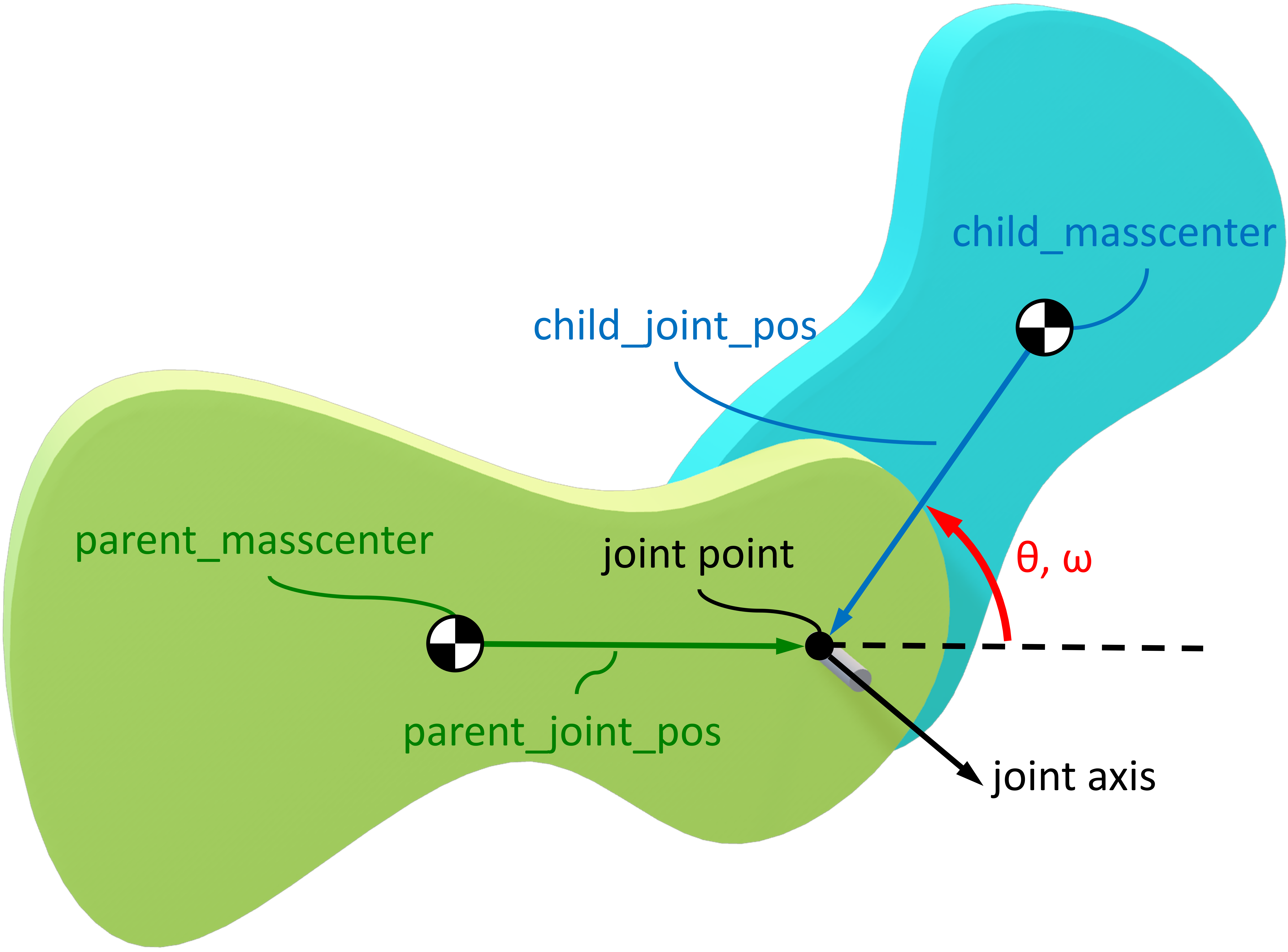
parent_joint_pos : Vector, optional

Vector from the parent body’s mass center to the point where the parent and child are connected. The default value is the zero vector.

child_joint_pos : Vector, optional

Vector from the child body’s mass center to the point where the parent and child are connected. The default value is the zero vector.

parent_axis : Vector, optional

Axis fixed in the parent body which aligns with an axis fixed in the child body. The default is x axis in parent’s reference frame.

child_axis : Vector, optional

Axis fixed in the child body which aligns with an axis fixed in the parent body. The default is x axis in child’s reference frame.

Explanation

A joint subtracts degrees of freedom from a body. This is the base class for all specific joints and holds all common methods acting as an interface for all joints. Custom joint can be created by inheriting Joint class and defining all abstract functions.

The abstract methods are:

_generate_coordinates
_generate_speeds
_orient_frames
_set_angular_velocity
_set_linar_velocity

Notes

The direction cosine matrix between the child and parent is formed using a simple rotation about an axis that is normal to both child_axis and parent_axis. In general, the normal axis is formed by crossing the child_axis into the parent_axis except if the child and parent axes are in exactly opposite directions. In that case the rotation vector is chosen using the rules in the following table where C is the child reference frame and P is the parent reference frame:

`child_axis`	`parent_axis`	`rotation_axis`
`-C.x`	`P.x`	`P.z`
`-C.y`	`P.y`	`P.x`
`-C.z`	`P.z`	`P.y`
`-C.x-C.y`	`P.x+P.y`	`P.z`
`-C.y-C.z`	`P.y+P.z`	`P.x`
`-C.x-C.z`	`P.x+P.z`	`P.y`
`-C.x-C.y-C.z`	`P.x+P.y+P.z`	`(P.x+P.y+P.z) × P.x`

Attributes

name	(string) The joint’s name.
parent	(Body) The joint’s parent body.
child	(Body) The joint’s child body.
coordinates	(list) List of the joint’s generalized coordinates.
speeds	(list) List of the joint’s generalized speeds.
parent_point	(Point) The point fixed in the parent body that represents the joint.
child_point	(Point) The point fixed in the child body that represents the joint.
parent_axis	(Vector) The axis fixed in the parent frame that represents the joint.
child_axis	(Vector) The axis fixed in the child frame that represents the joint.
kdes	(list) Kinematical differential equations of the joint.

property child#: Child body of Joint.

property child_axis#: The axis of child frame.

property child_point#: The joint’s point where child body is connected to the joint.

property coordinates#: List generalized coordinates of the joint.

property kdes#: Kinematical differential equations of the joint.

property parent#: Parent body of Joint.

property parent_axis#: The axis of parent frame.

property parent_point#: The joint’s point where parent body is connected to the joint.

property speeds#: List generalized coordinates of the joint..

PinJoint#

class sympy.physics.mechanics.joint.PinJoint(name, parent, child, coordinates=None, speeds=None, parent_joint_pos=None, child_joint_pos=None, parent_axis=None, child_axis=None)[source]#

Pin (Revolute) Joint.

Parameters:

name : string

A unique name for the joint.

parent : Body

The parent body of joint.

child : Body

The child body of joint.

coordinates: dynamicsymbol, optional

Generalized coordinates of the joint.

speeds : dynamicsymbol, optional

Generalized speeds of joint.

parent_joint_pos : Vector, optional

Vector from the parent body’s mass center to the point where the parent and child are connected. The default value is the zero vector.

child_joint_pos : Vector, optional

Vector from the child body’s mass center to the point where the parent and child are connected. The default value is the zero vector.

parent_axis : Vector, optional

Axis fixed in the parent body which aligns with an axis fixed in the child body. The default is x axis in parent’s reference frame.

child_axis : Vector, optional

Axis fixed in the child body which aligns with an axis fixed in the parent body. The default is x axis in child’s reference frame.

Explanation

A pin joint is defined such that the joint rotation axis is fixed in both the child and parent and the location of the joint is relative to the mass center of each body. The child rotates an angle, θ, from the parent about the rotation axis and has a simple angular speed, ω, relative to the parent. The direction cosine matrix between the child and parent is formed using a simple rotation about an axis that is normal to both child_axis and parent_axis, see the Notes section for a detailed explanation of this.

Examples

A single pin joint is created from two bodies and has the following basic attributes:

>>> from sympy.physics.mechanics import Body, PinJoint
>>> parent = Body('P')
>>> parent
P
>>> child = Body('C')
>>> child
C
>>> joint = PinJoint('PC', parent, child)
>>> joint
PinJoint: PC  parent: P  child: C
>>> joint.name
'PC'
>>> joint.parent
P
>>> joint.child
C
>>> joint.parent_point
PC_P_joint
>>> joint.child_point
PC_C_joint
>>> joint.parent_axis
P_frame.x
>>> joint.child_axis
C_frame.x
>>> joint.coordinates
[theta_PC(t)]
>>> joint.speeds
[omega_PC(t)]
>>> joint.child.frame.ang_vel_in(joint.parent.frame)
omega_PC(t)*P_frame.x
>>> joint.child.frame.dcm(joint.parent.frame)
Matrix([
[1,                 0,                0],
[0,  cos(theta_PC(t)), sin(theta_PC(t))],
[0, -sin(theta_PC(t)), cos(theta_PC(t))]])
>>> joint.child_point.pos_from(joint.parent_point)
0

To further demonstrate the use of the pin joint, the kinematics of simple double pendulum that rotates about the Z axis of each connected body can be created as follows.

>>> from sympy import symbols, trigsimp
>>> from sympy.physics.mechanics import Body, PinJoint
>>> l1, l2 = symbols('l1 l2')

First create bodies to represent the fixed ceiling and one to represent each pendulum bob.

>>> ceiling = Body('C')
>>> upper_bob = Body('U')
>>> lower_bob = Body('L')

The first joint will connect the upper bob to the ceiling by a distance of l1 and the joint axis will be about the Z axis for each body.

>>> ceiling_joint = PinJoint('P1', ceiling, upper_bob,
... child_joint_pos=-l1*upper_bob.frame.x,
... parent_axis=ceiling.frame.z,
... child_axis=upper_bob.frame.z)

The second joint will connect the lower bob to the upper bob by a distance of l2 and the joint axis will also be about the Z axis for each body.

>>> pendulum_joint = PinJoint('P2', upper_bob, lower_bob,
... child_joint_pos=-l2*lower_bob.frame.x,
... parent_axis=upper_bob.frame.z,
... child_axis=lower_bob.frame.z)

Once the joints are established the kinematics of the connected bodies can be accessed. First the direction cosine matrices of pendulum link relative to the ceiling are found:

>>> upper_bob.frame.dcm(ceiling.frame)
Matrix([
[ cos(theta_P1(t)), sin(theta_P1(t)), 0],
[-sin(theta_P1(t)), cos(theta_P1(t)), 0],
[                0,                0, 1]])
>>> trigsimp(lower_bob.frame.dcm(ceiling.frame))
Matrix([
[ cos(theta_P1(t) + theta_P2(t)), sin(theta_P1(t) + theta_P2(t)), 0],
[-sin(theta_P1(t) + theta_P2(t)), cos(theta_P1(t) + theta_P2(t)), 0],
[                              0,                              0, 1]])

The position of the lower bob’s masscenter is found with:

>>> lower_bob.masscenter.pos_from(ceiling.masscenter)
l1*U_frame.x + l2*L_frame.x

The angular velocities of the two pendulum links can be computed with respect to the ceiling.

>>> upper_bob.frame.ang_vel_in(ceiling.frame)
omega_P1(t)*C_frame.z
>>> lower_bob.frame.ang_vel_in(ceiling.frame)
omega_P1(t)*C_frame.z + omega_P2(t)*U_frame.z

And finally, the linear velocities of the two pendulum bobs can be computed with respect to the ceiling.

>>> upper_bob.masscenter.vel(ceiling.frame)
l1*omega_P1(t)*U_frame.y
>>> lower_bob.masscenter.vel(ceiling.frame)
l1*omega_P1(t)*U_frame.y + l2*(omega_P1(t) + omega_P2(t))*L_frame.y

Attributes

name	(string) The joint’s name.
parent	(Body) The joint’s parent body.
child	(Body) The joint’s child body.
coordinates	(list) List of the joint’s generalized coordinates.
speeds	(list) List of the joint’s generalized speeds.
parent_point	(Point) The point fixed in the parent body that represents the joint.
child_point	(Point) The point fixed in the child body that represents the joint.
parent_axis	(Vector) The axis fixed in the parent frame that represents the joint.
child_axis	(Vector) The axis fixed in the child frame that represents the joint.
kdes	(list) Kinematical differential equations of the joint.

PrismaticJoint#

class sympy.physics.mechanics.joint.PrismaticJoint(name, parent, child, coordinates=None, speeds=None, parent_joint_pos=None, child_joint_pos=None, parent_axis=None, child_axis=None)[source]#

Prismatic (Sliding) Joint.

Parameters:

name : string

A unique name for the joint.

parent : Body

The parent body of joint.

child : Body

The child body of joint.

coordinates: dynamicsymbol, optional

Generalized coordinates of the joint.

speeds : dynamicsymbol, optional

Generalized speeds of joint.

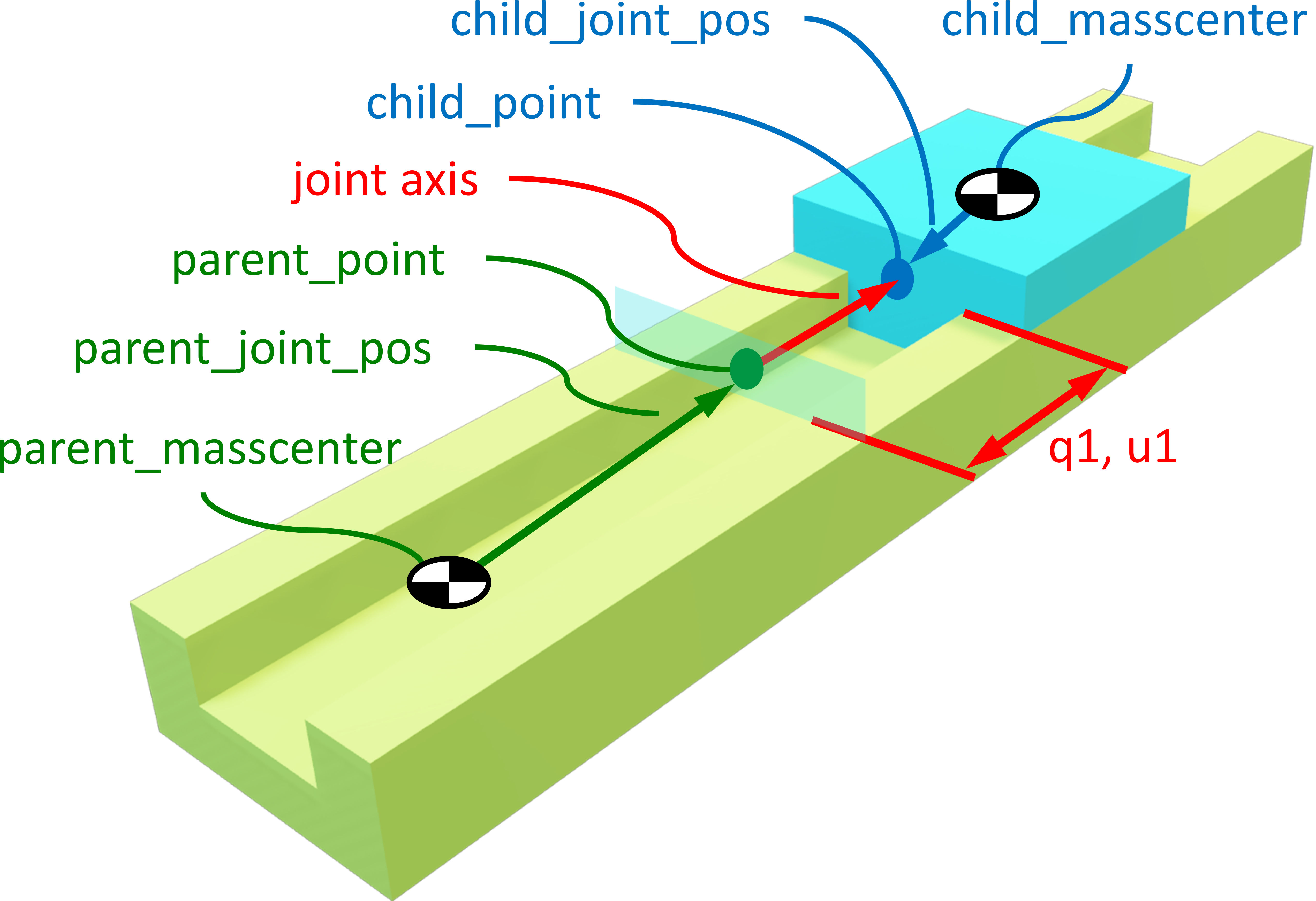
parent_joint_pos : Vector, optional

Vector from the parent body’s mass center to the point where the parent and child are connected. The default value is the zero vector.

child_joint_pos : Vector, optional

Vector from the child body’s mass center to the point where the parent and child are connected. The default value is the zero vector.

parent_axis : Vector, optional

Axis fixed in the parent body which aligns with an axis fixed in the child body. The default is x axis in parent’s reference frame.

child_axis : Vector, optional

Axis fixed in the child body which aligns with an axis fixed in the parent body. The default is x axis in child’s reference frame.

Explanation

It is defined such that the child body translates with respect to the parent body along the body fixed parent axis. The location of the joint is defined by two points in each body which coincides when the generalized coordinate is zero. The direction cosine matrix between the child and parent is formed using a simple rotation about an axis that is normal to both child_axis and parent_axis, see the Notes section for a detailed explanation of this.

Examples

A single prismatic joint is created from two bodies and has the following basic attributes:

>>> from sympy.physics.mechanics import Body, PrismaticJoint
>>> parent = Body('P')
>>> parent
P
>>> child = Body('C')
>>> child
C
>>> joint = PrismaticJoint('PC', parent, child)
>>> joint
PrismaticJoint: PC  parent: P  child: C
>>> joint.name
'PC'
>>> joint.parent
P
>>> joint.child
C
>>> joint.parent_point
PC_P_joint
>>> joint.child_point
PC_C_joint
>>> joint.parent_axis
P_frame.x
>>> joint.child_axis
C_frame.x
>>> joint.coordinates
[x_PC(t)]
>>> joint.speeds
[v_PC(t)]
>>> joint.child.frame.ang_vel_in(joint.parent.frame)
0
>>> joint.child.frame.dcm(joint.parent.frame)
Matrix([
[1, 0, 0],
[0, 1, 0],
[0, 0, 1]])
>>> joint.child_point.pos_from(joint.parent_point)
x_PC(t)*P_frame.x

To further demonstrate the use of the prismatic joint, the kinematics of two masses sliding, one moving relative to a fixed body and the other relative to the moving body. about the X axis of each connected body can be created as follows.

>>> from sympy.physics.mechanics import PrismaticJoint, Body

First create bodies to represent the fixed ceiling and one to represent a particle.

>>> wall = Body('W')
>>> Part1 = Body('P1')
>>> Part2 = Body('P2')

The first joint will connect the particle to the ceiling and the joint axis will be about the X axis for each body.

>>> J1 = PrismaticJoint('J1', wall, Part1)

The second joint will connect the second particle to the first particle and the joint axis will also be about the X axis for each body.

>>> J2 = PrismaticJoint('J2', Part1, Part2)

Once the joint is established the kinematics of the connected bodies can be accessed. First the direction cosine matrices of Part relative to the ceiling are found:

>>> Part1.dcm(wall)
Matrix([
[1, 0, 0],
[0, 1, 0],
[0, 0, 1]])

>>> Part2.dcm(wall)
Matrix([
[1, 0, 0],
[0, 1, 0],
[0, 0, 1]])

The position of the particles’ masscenter is found with:

>>> Part1.masscenter.pos_from(wall.masscenter)
x_J1(t)*W_frame.x

>>> Part2.masscenter.pos_from(wall.masscenter)
x_J1(t)*W_frame.x + x_J2(t)*P1_frame.x

The angular velocities of the two particle links can be computed with respect to the ceiling.

>>> Part1.ang_vel_in(wall)
0

>>> Part2.ang_vel_in(wall)
0

And finally, the linear velocities of the two particles can be computed with respect to the ceiling.

>>> Part1.masscenter_vel(wall)
v_J1(t)*W_frame.x

>>> Part2.masscenter.vel(wall.frame)
v_J1(t)*W_frame.x + Derivative(x_J2(t), t)*P1_frame.x

Attributes

name	(string) The joint’s name.
parent	(Body) The joint’s parent body.
child	(Body) The joint’s child body.
coordinates	(list) List of the joint’s generalized coordinates.
speeds	(list) List of the joint’s generalized speeds.
parent_point	(Point) The point fixed in the parent body that represents the joint.
child_point	(Point) The point fixed in the child body that represents the joint.
parent_axis	(Vector) The axis fixed in the parent frame that represents the joint.
child_axis	(Vector) The axis fixed in the child frame that represents the joint.
kdes	(list) Kinematical differential equations of the joint.

JointsMethod (Docstring)#

class sympy.physics.mechanics.jointsmethod.JointsMethod(newtonion, *joints)[source]#

Method for formulating the equations of motion using a set of interconnected bodies with joints.

Parameters:

newtonion : Body or ReferenceFrame

The newtonion(inertial) frame.

*joints : Joint

The joints in the system

Examples

This is a simple example for a one degree of freedom translational spring-mass-damper.

>>> from sympy import symbols
>>> from sympy.physics.mechanics import Body, JointsMethod, PrismaticJoint
>>> from sympy.physics.vector import dynamicsymbols
>>> c, k = symbols('c k')
>>> x, v = dynamicsymbols('x v')
>>> wall = Body('W')
>>> body = Body('B')
>>> J = PrismaticJoint('J', wall, body, coordinates=x, speeds=v)
>>> wall.apply_force(c*v*wall.x, reaction_body=body)
>>> wall.apply_force(k*x*wall.x, reaction_body=body)
>>> method = JointsMethod(wall, J)
>>> method.form_eoms()
Matrix([[-B_mass*Derivative(v(t), t) - c*v(t) - k*x(t)]])
>>> M = method.mass_matrix_full
>>> F = method.forcing_full
>>> rhs = M.LUsolve(F)
>>> rhs
Matrix([
[                     v(t)],
[(-c*v(t) - k*x(t))/B_mass]])

Notes

JointsMethod currently only works with systems that do not have any configuration or motion constraints.

Attributes

q, u	(iterable) Iterable of the generalized coordinates and speeds
bodies	(iterable) Iterable of Body objects in the system.
loads	(iterable) Iterable of (Point, vector) or (ReferenceFrame, vector) tuples describing the forces on the system.
mass_matrix	(Matrix, shape(n, n)) The system’s mass matrix
forcing	(Matrix, shape(n, 1)) The system’s forcing vector
mass_matrix_full	(Matrix, shape(2n, 2n)) The “mass matrix” for the u’s and q’s
forcing_full	(Matrix, shape(2*n, 1)) The “forcing vector” for the u’s and q’s
method	(KanesMethod or Lagrange’s method) Method’s object.
kdes	(iterable) Iterable of kde in they system.

property bodies#: List of bodies in they system.

property forcing#: The system’s forcing vector.

property forcing_full#: The “forcing vector” for the u’s and q’s.

form_eoms(method=<class 'sympy.physics.mechanics.kane.KanesMethod'>)[source]#

Method to form system’s equation of motions.

Parameters:: method : Class

Class name of method.
Returns:: Matrix

Vector of equations of motions.

Examples

This is a simple example for a one degree of freedom translational spring-mass-damper.

>>> from sympy import S, symbols
>>> from sympy.physics.mechanics import LagrangesMethod, dynamicsymbols, Body
>>> from sympy.physics.mechanics import PrismaticJoint, JointsMethod
>>> q = dynamicsymbols('q')
>>> qd = dynamicsymbols('q', 1)
>>> m, k, b = symbols('m k b')
>>> wall = Body('W')
>>> part = Body('P', mass=m)
>>> part.potential_energy = k * q**2 / S(2)
>>> J = PrismaticJoint('J', wall, part, coordinates=q, speeds=qd)
>>> wall.apply_force(b * qd * wall.x, reaction_body=part)
>>> method = JointsMethod(wall, J)
>>> method.form_eoms(LagrangesMethod)
Matrix([[b*Derivative(q(t), t) + k*q(t) + m*Derivative(q(t), (t, 2))]])

We can also solve for the states using the ‘rhs’ method.

>>> method.rhs()
Matrix([
[                Derivative(q(t), t)],
[(-b*Derivative(q(t), t) - k*q(t))/m]])

property kdes#: List of the generalized coordinates.

property loads#: List of loads on the system.

property mass_matrix#: The system’s mass matrix.

property mass_matrix_full#: The “mass matrix” for the u’s and q’s.

property method#: Object of method used to form equations of systems.

property q#: List of the generalized coordinates.

rhs(inv_method=None)[source]#

Returns equations that can be solved numerically.

Parameters:: inv_method : str

The specific sympy inverse matrix calculation method to use. For a list of valid methods, see inv()
Returns:: Matrix

Numerically solveable equations.